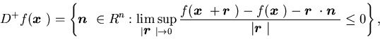
To more precisely state their results, we need to specify the model
of a single/parallel machine manufacturing system. Following the notation
given by Sethi, Soner, Zhang, and Jiang (1992),
let ![]() ,
,![]() ,
,![]() ,
and m(t) denote, respectively, the inventory level, the production
rate, the demand rate, and the machine capacity level at time
,
and m(t) denote, respectively, the inventory level, the production
rate, the demand rate, and the machine capacity level at time ![]() .
We assume that
.
We assume that![]() ,
,![]() ,
,![]() is a constant positive vector in Rn+. Furthermore,
we assume that
is a constant positive vector in Rn+. Furthermore,
we assume that ![]() is a Markov process with a finite space
is a Markov process with a finite space ![]() .
.
We can now write the dynamics of the system as
|
|
(2.1) |
![$\displaystyle J({\mbox{\boldmath$x$ }},m, {\mbox{\boldmath$u$ }}(\cdot))=E\int^......ty}_0e^{-\rho t}[h({\mbox{\boldmath$x$ }}(t))+c({\mbox{\boldmath$u$ }}(t))]dt,$](img28.gif) |
(2.2) |
where ![]() is the given discount rate. The problem is to choose an admissible control
is the given discount rate. The problem is to choose an admissible control ![]() that minimizes the cost function
that minimizes the cost function![]() .
We define the value function as
.
We define the value function as
|
|
(2.3) |
We make the following assumptions on the cost functions![]() and
and ![]() .
.
Assumption 2.1![]() is a nonnegative, convex function with
h(0)=0. There are positive
constants C21, C22,
C23,
and
is a nonnegative, convex function with
h(0)=0. There are positive
constants C21, C22,
C23,
and ![]() ,
,![]() such that
such that
Assumption 2.2![]() is a nonnegative function, c(0)=0, and
is a nonnegative function, c(0)=0, and![]() is twice differentiable. Moreover,
is twice differentiable. Moreover, ![]() is either strictly convex or linear.
is either strictly convex or linear.
Assumption 2.3![]() is a finite state Markov chain with generator Q, where Q=(qij),
is a finite state Markov chain with generator Q, where Q=(qij), ![]() is a(p+1) x (p+1) matrix
such that
is a(p+1) x (p+1) matrix
such that ![]() for
for ![]() and
and ![]() .
That is, for any function
.
That is, for any function![]() on
on ![]() ,
,
![\begin{displaymath}Qf(\cdot)(m)=\sum_{\ell \neq m}q_{m\ell}[f(\ell)-f(m)].\end{displaymath}](img41.gif)
Theorem 2.1 (i)
For each m, ![]() is convex on Rn, and
is convex on Rn, and ![]() is strictly convex if
is strictly convex if ![]() is so. (ii) There exist positive constants C24, C25,
and C26 such that for each m
is so. (ii) There exist positive constants C24, C25,
and C26 such that for each m
where ![]() and
and ![]() are the power indices in Assumption 2.1.
are the power indices in Assumption 2.1.
We next consider the equation associated with the problem. To do this, let
|
|
(2.4) |
In general, the value function v may not be differentiable. In
order to make sense of the HJB equation (2.4),
we consider its viscosity solution. In order to give the definition
of the viscosity solution, we first introduce the superdifferential and
subdifferential of a given function ![]() on Rn.
on Rn.
Definition 2.3 The superdifferential ![]() and the subdifferential
and the subdifferential![]() of any function
of any function ![]() on Rn are defined, respectively, as follows:
on Rn are defined, respectively, as follows:
Definition 2.4 We say that![]() is a viscosity solution of equation (2.4)
if the following holds:
is a viscosity solution of equation (2.4)
if the following holds:
Lehoczky, Sethi, Soner, and Taksar (1991) prove the following theorem.
Theorem 2.2 The value function ![]() defined in (2.3) is the unique viscosity
solution to the HJB equation (2.4).
defined in (2.3) is the unique viscosity
solution to the HJB equation (2.4).
Remark 2.1 If there is a continuously differentiable function that satisfies the HJB equation (2.4), then it is a viscosity solution, and therefore, it is the value function.
Furthermore, we have the following result.
Theorem 2.3 The value function ![]() is continuously differentiable and satisfies the HJB equation (2.4).
is continuously differentiable and satisfies the HJB equation (2.4).
For the proof, see Theorem 3.1 in Sethi and Zhang (1994a).
Next, we give a verification theorem.
Theorem 2.4 (Verification Theorem)
Suppose that there is a continuously differentiable function ![]() that satisfies the HJB equation (2.4).
If
there exists
that satisfies the HJB equation (2.4).
If
there exists ![]() ,
for which the corresponding
,
for which the corresponding![]() satisfies (2.1) with
satisfies (2.1) with![]() ,
,![]() ,
and
,
and
For the proof, see Lemma H.3 of Sethi and Zhang (1994a).
Next we give an application of the verification theorem. With Assumption 2.2, we can use the verification theorem to derive an optimal feedback control for n=1. From Theorem 2.4, an optimal feedback control u*(x,m) must minimize
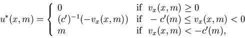
Recall that ![]() is a convex function. Thus u*(x,m) is increasing
in x. From a result on differential equations (see
Hartman
(1982)),
is a convex function. Thus u*(x,m) is increasing
in x. From a result on differential equations (see
Hartman
(1982)),
Next we will discuss the monotonicity of the turnpike set. To do this,
define ![]() to be such that i0<z<i0+1.
Observe that for
to be such that i0<z<i0+1.
Observe that for![]() ,
,
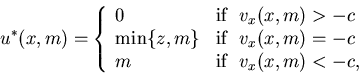
If the production cost is linear, i.e., c(u)=cu
for some constant c, then xm is the threshold
inventory level with capacity m. Specifically, if ![]() ,
and if
,
and if ![]() (full available capacity).
(full available capacity).
Let us make the following observation. If the capacity m>z,
then the optimal trajectory will move toward the turnpike set xm.
Suppose the inventory level is xm for some m and
the capacity increases to m1>m; it then becomes
costly to keep the inventory at level xm, since a lower
inventory level may be more desirable given the higher current capacity.
Thus, we expect ![]() .
Sethi,
Soner, Zhang, and Jiang (1992) show that this intuitive observation
is true. We state their result as the following theorem.
.
Sethi,
Soner, Zhang, and Jiang (1992) show that this intuitive observation
is true. We state their result as the following theorem.
Theorem 2.5 Assume ![]() to be differentiable and strictly convex. Then
to be differentiable and strictly convex. Then