Now we give the mathematically precise description of a jobshop suggested by Presman, Sethi, and Suo (1997a) as a revision of the description by Sethi and Zhang (1994a). First we give some definitions.
Definition 2.9 A manufacturing diagraph is
a graph![]() ,
where
,
where ![]() is a set of
is a set of ![]() ,
vertices,
and
,
vertices,
and ![]() is a set of ordered pairs called arcs, satisfying the following
properties:
is a set of ordered pairs called arcs, satisfying the following
properties:
Definition 2.10 In a manufacturing digraph, the source is called the supply node and the sink represents the customers. Vertices immediately preceding the sink are called external buffers, and all others are called internal buffers.
In order to obtain the system dynamics from a given manufacturing digraph,
a systematic procedure is required to label the state and control variables.
For this purpose, note that our manufacturing digraph ![]() contains a total of Nb+2 vertices including the source,
the sink, m internal buffers, and Nb-m
external buffers for some integer m and Nb,
contains a total of Nb+2 vertices including the source,
the sink, m internal buffers, and Nb-m
external buffers for some integer m and Nb, ![]() ,
,![]() .
.
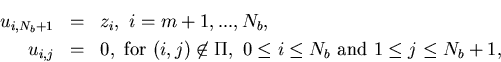
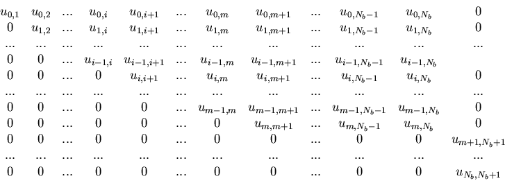
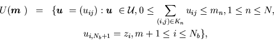
Theorem 2.8 We can label all the vertices from 0 to Nb+1 in a way so that the label numbers of the vertices along every path are in a strictly increasing order, the source is labeled 0, the sink is labeled Nb+1, and the external buffers are labeled m+1, m+2,...,Nb.
The proof is similar to Theorem 2.2 in Sethi, and Zhou (1994).
With the help of Theorem 2.8, one is able to formally write the dynamics and the state constraints associated with a given manufacturing digraph. To do this, we require the following definitions.
Definition 2.11 For each arc
(i,j), ![]() ,
in a manufacturing digraph, the rate at which parts in buffer i
are converted to parts in buffer j is labeled as controluij.
Moreover, the control uij associated with the arc (i,j)
is called an output of i and an input to j.
In particular, outputs of the source are called primary controls
of the digraph. For each arc (i, Nb+1),
i=m+1,...,Nb,
the demand for products in buffer i is denoted by zi.
,
in a manufacturing digraph, the rate at which parts in buffer i
are converted to parts in buffer j is labeled as controluij.
Moreover, the control uij associated with the arc (i,j)
is called an output of i and an input to j.
In particular, outputs of the source are called primary controls
of the digraph. For each arc (i, Nb+1),
i=m+1,...,Nb,
the demand for products in buffer i is denoted by zi.
In what follows, we shall also set
Definition 2.12 In a manufacturing
digraph ![]() ,
a set
,
a set![]() is called a placement of machines 1,2,...,N, if
is called a placement of machines 1,2,...,N, if ![]() is a partition of
is a partition of ![]() ,
namely,
,
namely, ![]() ,
,![]() for
for ![]() ,
and
,
and ![]() .
.
A dynamic jobshop can be uniquely specified by a triple![]() ,
which denotes a manufacturing system that corresponds to a manufacturing
digraph
,
which denotes a manufacturing system that corresponds to a manufacturing
digraph ![]() along with a placement of machines
along with a placement of machines ![]() .
.
Consider a jobshop ![]() ,
let
uij(t) be the control at time t associated
with arc (i,j),
,
let
uij(t) be the control at time t associated
with arc (i,j), ![]() .
Suppose we are given a stochastic process
.
Suppose we are given a stochastic process![]() on the standard probability space
on the standard probability space ![]() with
mn( t) representing the capacity of the nth
machine at time t, n=1,...,N. The controls
uij(t)
with
with
mn( t) representing the capacity of the nth
machine at time t, n=1,...,N. The controls
uij(t)
with ![]() ,
n=1,...,N,
,
n=1,...,N,![]() ,
should satisfy the following constraints:
,
should satisfy the following constraints:
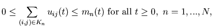 |
(2.12) |
We denote the surplus at time t in buffer i by
xi(t), ![]() .
Note that if xi(t)>0, i=1,...,Nb,
we have an inventory in buffer i, and if xi(t)<0,
i=m+1,...,Nb,
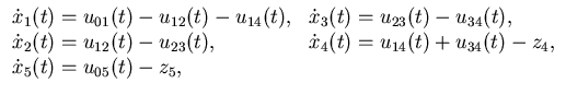
we have a shortage of finished product i. The dynamics of the system
are, therefore,
.
Note that if xi(t)>0, i=1,...,Nb,
we have an inventory in buffer i, and if xi(t)<0,
i=m+1,...,Nb,
we have a shortage of finished product i. The dynamics of the system
are, therefore,
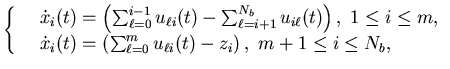 |
(2.13) |
 |
(2.14) |
|
|
(2.15) |
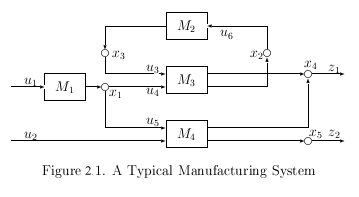
Let us illustrate a jobshop by the following simple example.
Example 2.1. In Figure 2.1, we have four machines ![]() ,
two distinct products, and five buffers. Each machine
,
two distinct products, and five buffers. Each machine ![]() has capacity
mi(t) at time t, and each
product j=1,2 has demand zj. As indicated in the
figure,
has capacity
mi(t) at time t, and each
product j=1,2 has demand zj. As indicated in the
figure, ![]() known as the state variables are associated with the buffers. More specifically,
xi
denotes the inventory/backlog of part type
known as the state variables are associated with the buffers. More specifically,
xi
denotes the inventory/backlog of part type![]() .
Control variables
.
Control variables ![]() represent production rates. More specifically, u 1 and
u2
are the rates at which raw parts coming from outside are converted to part
types 1 and 5, respectively, and u3,
u4,
u5
and u6 are the rates of conversion from part types 3,1,1,
and 2 to part types 4, 2, 4 and 3, respectively. Thus,
represent production rates. More specifically, u 1 and
u2
are the rates at which raw parts coming from outside are converted to part
types 1 and 5, respectively, and u3,
u4,
u5
and u6 are the rates of conversion from part types 3,1,1,
and 2 to part types 4, 2, 4 and 3, respectively. Thus,
 |
(2.16) |
| (2.17) |
|
|
(2.18) |
We are now in the position to formulate our stochastic optimal control
problem for the jobshop defined by (2.13)-(2.15).
For ![]() ,
let
,
let

Let ![]() denote the set of all admissible control with respect to
denote the set of all admissible control with respect to ![]() and the machine capacity vector
and the machine capacity vector ![]() .
The problem is to find an admissible control
.
The problem is to find an admissible control![]() that minimizes the cost function
that minimizes the cost function
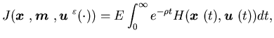 |
(2.19) |
The value function is then defined as
|
|
(2.20) |
Assumption 2.6![]() is a nonnegative and convex function. Further, for all
is a nonnegative and convex function. Further, for all ![]() and
and ![]() ,
there exist constants
,
there exist constants ![]() and
and ![]() such that
such that
Assumption 2.7 Let ![]() for some given integer
for some given integer ![]() .
The capacity process
.
The capacity process![]() ,
,![]() ,
is a finite state Markov chain with generator Q=(qkk')
such that
,
is a finite state Markov chain with generator Q=(qkk')
such that ![]() if
if ![]() and
and![]() .
Moreover, Q is irreducible.
.
Moreover, Q is irreducible.
We use ![]() to denote our control problem. Presman, Sethi,
and Suo (1997a) prove the following theorem.
to denote our control problem. Presman, Sethi,
and Suo (1997a) prove the following theorem.
Theorem 2.9 The optimal control ![]() exists, and can be represented as a feedback control, i.e., there exists
a function
exists, and can be represented as a feedback control, i.e., there exists
a function ![]() such that for any
such that for any ![]() we have
we have
Now we consider the Lipschitz property of the value function. It should
be noted that unlike in the case without state constraints, the Lipschitz
property in our case does not follow directly. The reason for this is that
in the presence of state constraints, a control which is admissible with
respect to ![]() is not necessarily admissible for
is not necessarily admissible for ![]() when
when![]() .
.
Theorem 2.10 The value function is convex and continuous, and satisfies the condition
|
|
(2.21) |
Because the problem of the jobshop involves state constraints, we can write the HJBDD for the problem as in Section 2.2:
|
|
(2.22) |
Theorem 2.11 (Verification Theorem)
(i) The value function![]() satisfies equation (2.22) for all
satisfies equation (2.22) for all![]() .
(ii) If some continuous convex function
.
(ii) If some continuous convex function ![]() satisfies (2.22)
and the growth condition
(2.21) with
satisfies (2.22)
and the growth condition
(2.21) with ![]() ,
then
,
then ![]() .
Moreover, if there exists a feedback control
.
Moreover, if there exists a feedback control ![]() providing the infimum in (2.22)
for
providing the infimum in (2.22)
for ![]() ,
then
,
then![]() ,
and
,
and ![]() is an optimal feedback control. (iii) Assume that
is an optimal feedback control. (iii) Assume that ![]() is strictly convex in
is strictly convex in ![]() for each fixed
for each fixed ![]() .
Let
.
Let ![]() denote the minimizer function of the right-hand side of (2.22).
Then,
denote the minimizer function of the right-hand side of (2.22).
Then,
Remark 2.6 The HJBDD (2.22)
coincides at inner points of ![]() with the usual dynamic programming equation for convex PDP problems. Here
PDP is the abbreviation of piecewise deterministic processes introduced
by Vermes (1985) and Davis
(1993). The HJBDD gives at boundary points of
with the usual dynamic programming equation for convex PDP problems. Here
PDP is the abbreviation of piecewise deterministic processes introduced
by Vermes (1985) and Davis
(1993). The HJBDD gives at boundary points of ![]() ,
a boundary condition in the following sense. Let the restriction of
,
a boundary condition in the following sense. Let the restriction of ![]() on some l-dimensional face, 0<l<N, of the boundary
of S be differentiable at an inner point
on some l-dimensional face, 0<l<N, of the boundary
of S be differentiable at an inner point ![]() of this face. Note that this restriction is convex and is differentiable
almost everywhere on this face. Then there is a vector
of this face. Note that this restriction is convex and is differentiable
almost everywhere on this face. Then there is a vector ![]() such that
such that ![]() for any admissible direction at
for any admissible direction at ![]() .
It follows from the continuity of the value function that
.
It follows from the continuity of the value function that
| + | |||
| = | (2.23) |
According to (2.22), optimal feedback control policies are obtained in terms of the directional derivatives of the value function.
Note now that the uniqueness of the optimal control follows directly
from the strict convexity of function ![]() in
in ![]() and the fact that any convex combination of admissible controls for any
given
and the fact that any convex combination of admissible controls for any
given ![]() is also admissible. For proving the remaining statements of Theorem
2.10 and Theorem 2.11, see Presman,
Sethi, and Suo (1997a).
is also admissible. For proving the remaining statements of Theorem
2.10 and Theorem 2.11, see Presman,
Sethi, and Suo (1997a).
Remark 2.7 Presman, Sethi, and Suo (1997a) show that Theorem 2.9, Theorem 2.10, and Theorem 2.11 also hold when the systems are subject to lower and upper bound constraints on work-in-process.